Binary search

#

Binary search is a better version of Linear search. Here, rather than checking each element one by one, we split the data structure in two halves and then compare our target with the middle element. But this comparison only makes sense if the data structure is either sorted in an ascending or a descending manner. Therefore -

The array must be sorted for binary search to work.

Now lets try to see how it works step by step -

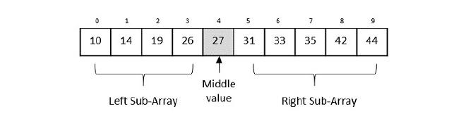
1. Let’s take an array for our example and try to understand what happens in Binary search. Let us suppose our target is 42.

2. First up, we have our starting index as 0 and our last index as n-1 (where n = total length of the array) and this is always the case with all arrays. This is where our search should happen.

3. Finding the mid value becomes easy now with the formula $$ (start+end)/2 $$ here this will be $$ (0+9)/2 = 4.5 = 4 $$(we will keep all parameters as int to make finding the middle easily.)

4. Now we can find the middle-most element as 27. Since array is sorted in an ascending order, we can see that our target is greater than the middle element hence we only need to search the right sub-array which contains elements larger than the center element

5. Now comes an important step. We have to change the start and end positions.

   • In case our target>middle element, we change the start as middle + 1
   • In case our target<middle element, we change the end to middle - 1
   • Otherwise target=middle In our case, we have target>middle, meaning we only have to search the right sub-tree so we need to change the start to middle+1, which will become, 4+1= 5. So now we will search from 5 to end (end is still the same, i.e. 9)

6. Repeat Step 3 and our middle index now becomes 7. The element at 7 is 35, i.e. target>middle element so start = middle +1. Now our start becomes 8. That means we will search from 8 to 9.

7. Repeat Step 3 and our middle index now becomes 8. This time when comparing the element at 8, we observe it is our target i.e. 42.

Similarly, we simply change the end to middle-1 in case we want to check the left sub-array and repeat the same process.

The code for the same in Python-

def binary_search(arr, x):
	start = 0
	end = len(arr) - 1
	 
	while (start <= end):
		mid = start + (end-start)/2
		if arr[mid] > x:
			end = mid - 1
		elif arr[mid] <x:
			start = mid + 1
		else:
			return mid
	return -1 #incase the target entered is not inside our array
	
arr = [10,14,19,26,27,31,33,35,42,44]
x = 42
result = binary_search(arr,x)

if result != -1:
	print("Element at index", result)
else:
	print("Element entered is not present in the array.")
	
	

Oops

#

Did you notice the formula I used to find the middle value in the above example? Well, If we think about it, calculating our middle index with the previous formula can be a bit tricky sometimes. Especially when both our start and end indices have very large values. By large, I mean large enough that sometimes, they can not be contained within certain data types (as every data type has a range. In C++, the range of int is -2,147,483,648 to 2,147,483,647). Now we may not reach these number of indices but our code is supposed to work for ALL kinds of data and there is a very simple way to avoid this problem.

Our problem occurs because we are supposedly adding 2 very large numbers whose sum can not be fit into our data type. But if we use the formula, $$ Mid = start + (end-start)/2$$ we are subtracting two huge numbers, dividing it by 2 and then adding a huge number which will not overflow our datatype! Also if simplify this formula, it’s basically a complicated way of writing the same thing but here, this gets our job done and not the simplified version so it’s better to use this instead of the previous one!

All the topics I’ll be covering in this blog are more or less related to the curriculum of my college. I might miss on some topics related to this topic. Feel free to reach out and let me know if I should add something else!

Merge Sort

#

A sorting algorithm based on the concept of Divide and conquer. Just like the previous algorithm, we divide our array into 2. The difference is, here we are sorting and not finding an element.

We keep dividing the array/vector/the linear data structure till each element is isolated. Then we backtrack and sort the small arrays and put them together ,hence the name. We divide the data structure and conquer the small portions and combine them together to be one big sorted data structure.

We use 2 major parts in this algorithm. One part is responsible for dividing the data structure multiple times till we reach individual elements and the other part is responsible for the sorting. Let’s see how it works step by step -

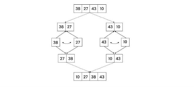
1. We have arr = [38,27,43,10]. First up we find the middle index. Mid = start + (end - start)/2 Mid = 0 + (3-0)/2 Mid = 1.5 = 1 (rounding off for our simplicity) So we have got Mid = arr[1] = 27 as the middle element

2. Now the array will be divided such that element after the middle element becomes is it’s own array.

3. We repeat this same process until we reach individual elements. For example the next step for the left sub-array would be- Mid = 0 + (1-0)/2 Mid = 0.5 = 0 Mid = arr[0] = 38 If we try to split this further, we have start and end both as ‘0’. Similarly for arr[1], we have start and end both equal to ‘1’. Hence no splitting can happen now and our divide step is over. Time for conquering! 👑

4. A major step is making our original data structure back from the small elements. Breaking is easy enough but putting them back in a sorted way? It might seem a bit confusing but it is quite easy once you understand what is happening. Let’s take an example - Imagine we have 2 arrays now - [27,38] and [10,43]. We need [10,27,38,47] but 10 is in the right sub-array… We shall use pointers to compare the values of each sub array with each other to get the result. 4.1 Put pointer i and j at the start of both the sub-arrays respectively. 4.2 Make a temporary array, temp, for example. So i = 0, j = 2(mid+1), temp = [] 4.3 Compare i and j. In our case, i = 27 and j = 10. j has a smaller element so we add 10 to temp and increase j by one so i= 0 , j = 3 and temp = [10] 4.4 Next we are comparing 27 and 43. Now i has a smaller element so we append the array with 27 and increase i by 1. That means - i =1, j= 3, temp = [10,27] We keep repeating this process until i and j go out of range. For the left sub-array, the range (for i) will end at mid + 1 and for the right sub-array, the range (for j) will end at end +1. Therefore, i<=mid and j <=end.

5. As we compare i and j, it is obvious that either i or j will cross their range and the comparison will stop. But what about the elements remaining in the sub-array which did not get added to temp? For example - In our case, we will get temp = [10,27,38] after performing 3 iterations of the comparison step (try to dry run and get the output!). But we still have the last element i.e. 43 in the right sub-array… In other cases, there can be a bunch of other elements remaining too. They will obviously be sorted as the sub-arrays will be sorted with our algo, but we need to store them in the temp array. So we will need another loop for this. (remember, in our case the right sub-array had left-over elements. It could also be that the left sub-array has such elements. So we need to create a loop for both the cases.)

6. Our final loop will put the elements from temp, to our original array. Also, if you tried to perform a dry run (very important!) and see the temp array, you will observe that the temp array’s index of an element is always start (of that sub-array) + index (of that element in that array) of what we want it to be in our final array so we will do - result[start + index] = temp[index] For e.g. [5,3] in temp. Let their indices be 2 and 3 respectively. In temp they will become [3,5] on indices 0 and 1 respectively. Now that 3 needs to go to the 2nd index of the actual array and 5 has to go to 3rd index. Notice, start = 2. If we add start to their indices of temp, i.e., 0 and 1, we get 2 and 3 that is what their place should be!

Let’s look at the code for the same -

def merge(arr, start, mid, end):
    temp = []
    i = start
    j = mid + 1

    while i <= mid and j <= end:
        if arr[i] <= arr[j]:
            temp.append(arr[i])
            i += 1
        else:
            temp.append(arr[j])
            j += 1

    # Remaining elements of left subarray
    while i <= mid:
        temp.append(arr[i])
        i += 1

    # Remaining elements of right subarray
    while j <= end:
        temp.append(arr[j])
        j += 1

    # Copy sorted temp back into original array
    for k in range(len(temp)):
        arr[start + k] = temp[k]


def mergeSort(arr, start, end):
    if start < end:
        mid = start + (end - start) // 2

        mergeSort(arr, start, mid)
        mergeSort(arr, mid + 1, end)

        merge(arr, start, mid, end)


arr = [3, 2, 6, 4, 1, 8]
mergeSort(arr, 0, len(arr) - 1)

for i in arr:
    print(i, end=' ')

By changing if arr[i] <= arr[j]: to if arr[i] >= arr[j]:, we can change the sorting to descending

Time complexity

#

The time complexity for this algorithm is O(nlogn) n for the merging step and logn for the division of elements. n being the number of elements in the data structure of course.

Space complexity

#

Is going to be n as the temp array that we create is an intermediate data structure that takes up space.

Quick sort

#

This sorting algorithm is based on the concept of pivot and partition. Pivot is basically an element that we select and compare with the rest of the elements and store them according to the problem to sort it either is an ascending manner or descending manner. We bring the pivot element at the center and hence do a partition of the data structure in a sense, hence the name.

Just like before, we divide the work in two major steps - Partitioning and the sorting of elements. Let’s understand with the help of an example -

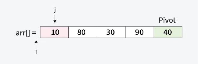
1. We will first think about dividing the the array. We need a pivot for that. The pivot can be the first element, the last element, the middlemost element or any random element as such. We will take the last element as our pivot.

2. Now we need put the smaller elements on the left side (assuming we are sorting in an ascending manner). That means the left half will go from the start of the array till pivot-1 (because pivot is at the center). And the right half will go from pivot+1 to end of the array. But how will we get the pivot to the center?

3. This is our second part of the problem. It’s very simple. We compare each element to the pivot and move the smaller elements in the beginning of the array. For this, we will use pointers. Since we need to compare each element (except of course the pivot) with the pivot, the loop should run from the start of the array to end-1 (because pivot is the ending element).

4. We will use a pointer, say i, at -1 (we will see why it is put at -1) and another pointer, say j that will compare elements to pivot. Remember, j will be increased till the pivot is reached.

5. Whenever we encounter an element which is smaller that the pivot, we will increase the value of i by 1 and swap the elements pointed by i and j. Using the example, we know 10 is smaller than 40, i =-1 and j = 0, arr[-1] = invalid, arr[0] = 10 Increasing the value of i and swapping them we will get - i = 0, j = 0, arr[0] = 10; meaning 10 is already to the left of pivot. Next up, j will be increased by one so i = 0, j = 1 and arr[j]=80>pivot therefore nothing will happen. Next up, j will be increased by one so i = 0, j = 2 and arr[j]=30 is smaller than pivot, so we will increase i by one and swap - i = 1, j = 2 and arr[j]=30, arr[1]= 80. After swap - [10,30,80,90,40]

6. Now we after repeating this (try dry run!) we will see our array will remain the same as all the elements smaller than pivot are already on the left of the array. But the pivot is still not in the center… Well if you did the dry run, you will see that i = 1 after comparing every element and all the elements smaller elements are on the left. What does that mean? That the next element that would be placed in the array would be the pivot! Yes! That means pivot would be placed at i+1 = 2. That means we will get arr=[10,30,40,90,80]

7. What now? Well we can partition the right half using the function we talked about earlier recursively (using 80 as pivot in the partition of [90,80], and swap the numbers again!)

Code

#

def swap(arr, i, j):
    arr[i], arr[j] = arr[j], arr[i]
    
def partition(arr, start, end):
    pivot = arr[end]
    i = start - 1
    
    for j in range(start, end):
        if arr[j] < pivot:
            i += 1
            swap(arr, i, j)
    
    #pivot at center
    i += 1
    swap(arr, i, end)
    
    return i

def quickSort(arr, start, end):
    if start < end:
        pivotIdx = partition(arr, start, end)
        quickSort(arr, start, pivotIdx - 1)
        quickSort(arr, pivotIdx + 1, end)

arr = [10, 80, 30, 90, 40]
quickSort(arr, 0, len(arr) - 1)
print(arr)

Just like before, we can change the less than sign to greater than sign to change the ordering to descending order. Try it yourself!

Time complexity

#

The average case time complexity is the same as Merge sort, i.e. O(nlogn) but if we see the worst case then it would become O(n^2).

This happens when we have pivot as smallest or largest element. For e.g. in [10,20,30,40,50], we set 50 as pivot. After taking n turns, we find out all elements are already arranged ascendingly. Then the array will get partitioned (there will be no right sub-array as all elements are smaller than 50). This same process will repeat. Mathematically, it forms an ap (n+[n-1] + [n-2] + ….), whose sum would be n*(n+1)/2 => O(n^2)

The space complexity is O(1) as there is no intermediate data structure (ignoring the recursion call stack). Hence in problems related to space complexity importance, we use this over Merge Sort.

Kadane’s Algorithm

#

This algorithm is used to solve the problem of maximum subarray sum. This problem has an array and our job is to find the subarray with the greatest sum. We have two ways to solve this problem. We can either brute force our way through. We do this by making a ‘sum’ variable where we store the sum of the elements which will keep increasing. The largest sum will become the ‘max_value’. After each iteration we will will compare the sum of the new subarray with the ‘max_value’ and change it’s value if we find a higher value. The worst case time complexity for this would be O(n^2) which is not the best… so we use Kadane’s Algorithm

We use one simple rule to optimize our previous appraoch. Since we want the highest sum, we can achieve that by NOT adding any large negative values to our sum. We will simple make the value of our sum to 0 once it’s value gets less than 0. Let’s see it working in code

Let’s assume our array to be arr= [2, 3, -8, 7, -1, 2, 3]

def kadaneAlgo(arr):
	currSum = 0
	maxSum = 0
	for i in range (0,len(arr)):
		currSum += i;
		maxSum = max(currSum, maxSum)
		
		if (currSum<0):
			currSum = 0
 
arr = [2, 3, -8, 7, -1, 2, 3]
    print(maxSubarraySum(arr))

Output - 11

The time complexity is O(n) which is wayyy better than the brute force method! This is also an example of dynamic programming algorithm as we solve one section of the problem (here, one subarray) at a time and it keeps increasing and the answer of the small subarrays give us the final answer at the end.